Part 1: Fun with Filters
Part 1.1: Convolutions from Scratch!
Naive approach with 4 for loops
def convovle_4(img, kernel,  mode='constant'):
    h,w = img.shape
    kernel = np.flip(kernel, (0, 1)) #flip the kernel
    k_h, k_w = kernel.shape
    convolved_img = np.copy(img)
    # padding
    pad_w= (k_w - 1) // 2
    pad_h = (k_h - 1) // 2
    img = np.pad(img, pad_width=((pad_h, pad_h), (pad_w, pad_w)), mode=mode)

    for i in range(w):
        for j in range(h):
            convolved_img[j][i] = 0
            for p in range(-pad_w, pad_w + 1):
                for q in range(-pad_h, pad_h + 1):
                    convolved_img[j][i] += kernel[q + pad_h][p + pad_w] * img[j + q + pad_h][i + p + pad_w]
    return convolved_img
Naive approach with 2 for loops
def patch(img, i, j, kw, kh):
    pad_w = (kw - 1) //2
    pad_h = (kh - 1) //2
    return img[j -pad_h:j+pad_h+1, i -pad_w:i+pad_w+1]

def convovle_2(img, kernel, mode='constant'):
    h,w = img.shape
    kernel = np.flip(kernel, (0, 1)) #flip the kernel
    k_h, k_w = kernel.shape
    convolved_img = np.copy(img)
    # zero padding
    pad_w= (k_w - 1) // 2
    pad_h = (k_h - 1) // 2

    img = np.pad(img, pad_width=((pad_h, pad_h), (pad_w, pad_w)), mode=mode)
    kernel_flat = kernel.ravel()
    for i in range(w):
        for j in range(h):
            curr_patch = patch(img, i+pad_w, j+pad_h, k_w, k_h)
            curr_patch_flat = curr_patch.ravel()
            convolved_img[j][i] = curr_patch_flat @ kernel_flat
    return convolved_img
The following is the code to construct kernels
                box_filter_9 = 1/81 * np.ones((9,9))
                Dx = np.array([[1, 0, -1]])
                Dy = np.array([[1], [0], [-1]])
The convolution with 4 for loops takes 18 seconds to run.
The convolution with 2 for loops takes 0.8 seconds to run.
The scipy_convovle_img = signal.convolve2d(im, box_filter_9, mode='same')
takes 0.1 seconds to run.
The less for loop we have in the implementation, the faster the convolution is.
I used zero-padding to handle boundary. To apply kernel the pixels on the boundary,
I manually add (kernel_width - 1) // 2 pixels with zero values on left and right side, and
(kernel_height - 1) // 2 zero-value pixels for top and bottom.

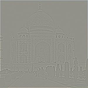
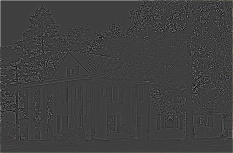
Part 1.2: Finite Difference Operator
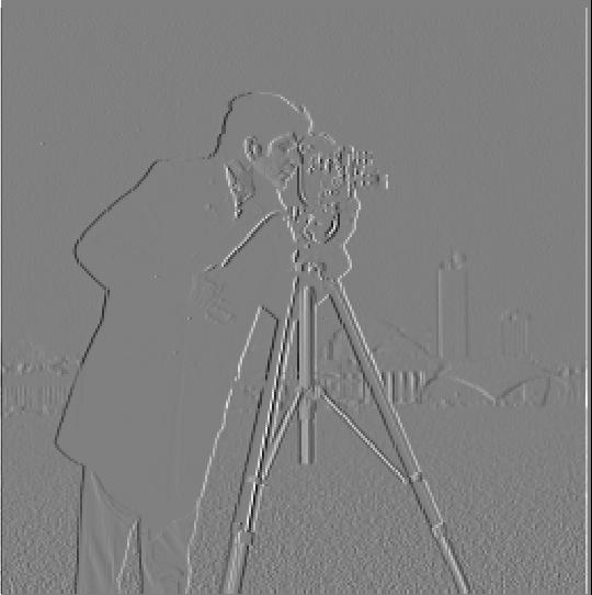
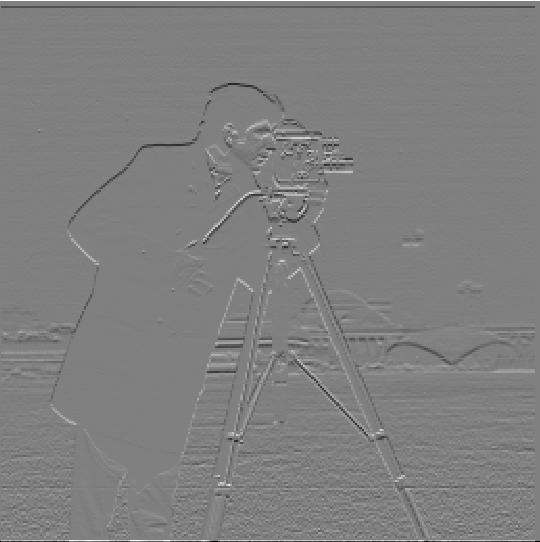
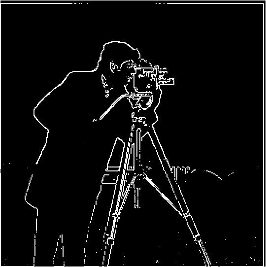
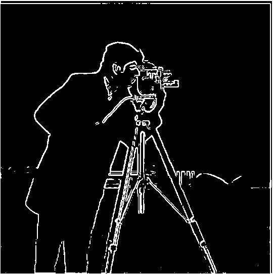
For binary edge image, to remove most of noise in the background, I chose threshold = 0.3. This will make image lost most edges in the buildings in the background and weaker edge on cameraman. But this threshold can remove most noise in the sky and land. This threshold can make sure I get most camerman edges with little noise.
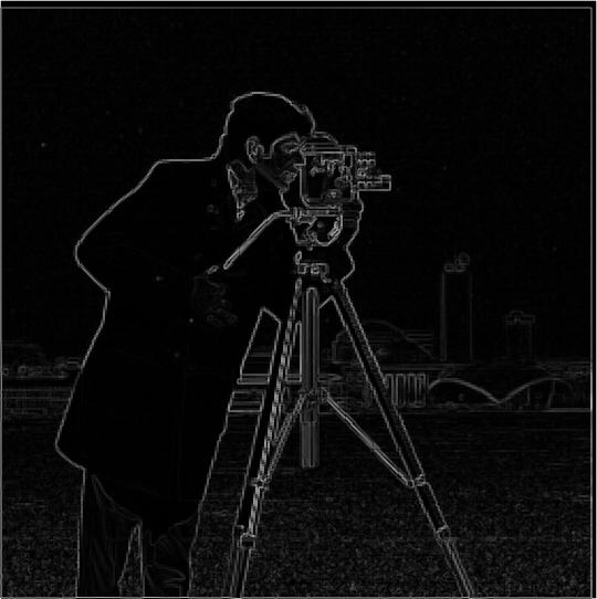
Part 1.3: Derivative of Gaussian (DoG) Filter
One way to create DoG filter: Convolve the gaussian kernel with D_x and D_y. The other way is create a blurred version of the original image by convolving with a gaussian and then apply Dx and Dy on the blured image then create binary edge image.
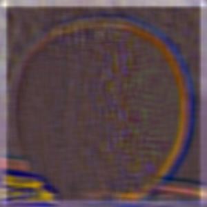
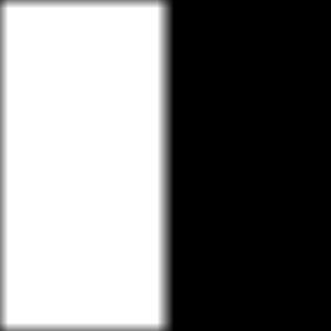
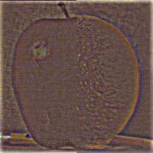
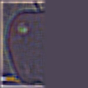
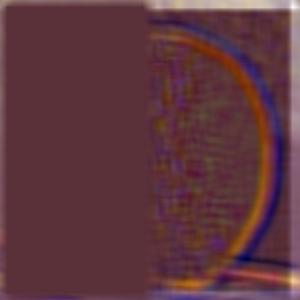
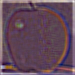
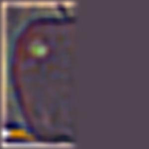
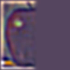
Here is visualization of DoG filter with Dx and Dy filter. To make effect obvious I used kernel size (70,70) and sigma 30


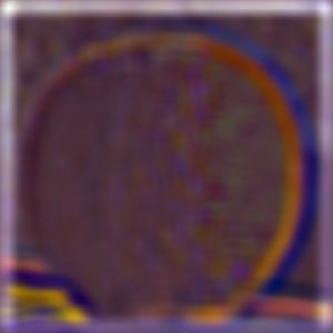
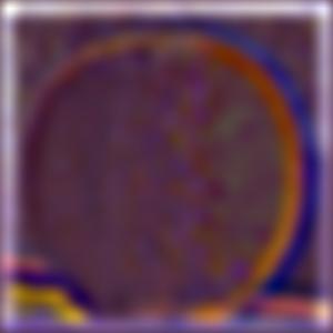
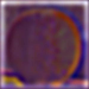
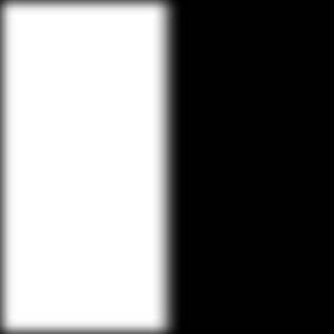
Visualization for kernel size (3,3) and sigma 1, this the kernel I actually used for DoG filter implementation

From above images, we can see using DoG filter we can remove most of noise in the background and preserve the main edges of cameraman. Using DoG filter can remove more noise and preserve more detail than using Finite Difference Operator directly.
Using DoG filter to create bineary edge with one convolution and blurring image then apply Dx Dy on the blurred image can create same output image.
Part 2.1: Image "Sharpening"
implemenet the gaussian kernel then convolve image with the kernel gave us the blurring/low-pass filter function
                        g1d = cv2.getGaussianKernel(3,1)
                        g2d = np.outer(g1d, g1d)
                        def blur_image_color(img, kernel):
                            img_channels = []
                            for i in range(3):
                                img_c = img[:,:,i]
                                sharpened_img_c = signal.convolve2d(img_c, kernel, mode='same')
                                img_channels.append(sharpened_img_c)
                            img = np.dstack(img_channels)
                            return img
                        blur_image_color(img, g2d)
To sharpen the image, you will need apply unsharp mask filter(gaussian filter) to create an image with low frequency and get high frequency image by subtracting low frequency image from original image. Then you add high frequency image back to original image to increase the intensity of the edge of high frequency and create sharpening effect. As a result, we get unsharp mask filter.

Using the formula above, we can finish sharpening in one convolution and can change sharpen intensity by changing alpha The higher the alpha value is,the stronger the sharpening effect is. Where f is the image, g is gaussian kernel, e is identity kernel, alpha is constant.

obseravtion
By trying to blur the image and resharpen it, we can see it loses some details after resharpen. After resharp, we can see noise around the edges of the buildings because we overlap too many high frequency values. So resharpend image sometimes can't reproduce the origianl image.
Part 2.2: Hybrid Images
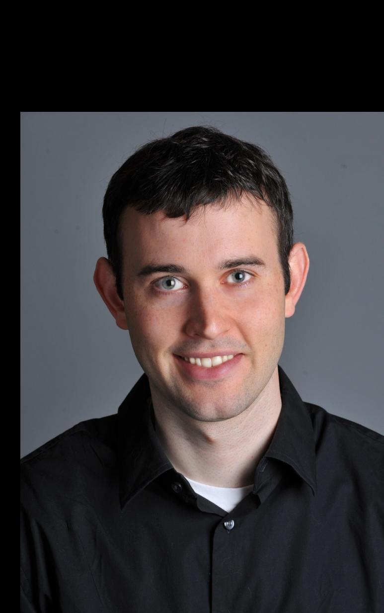
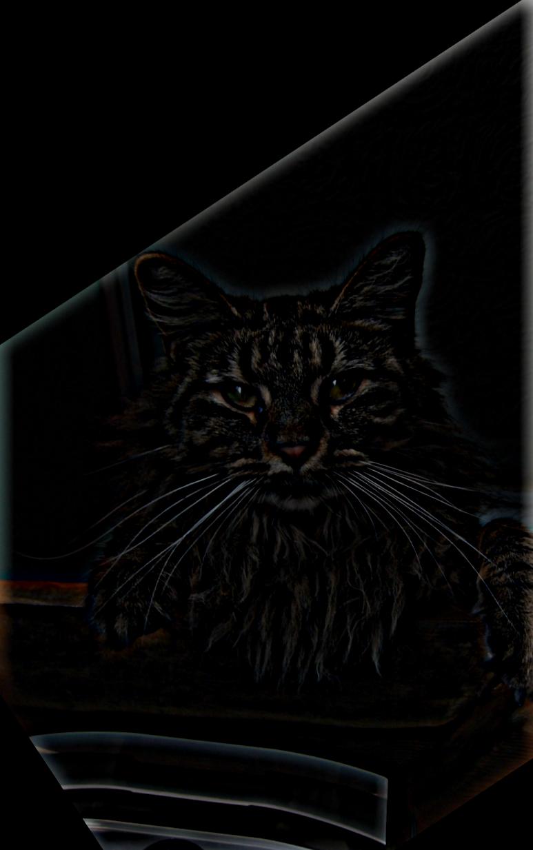
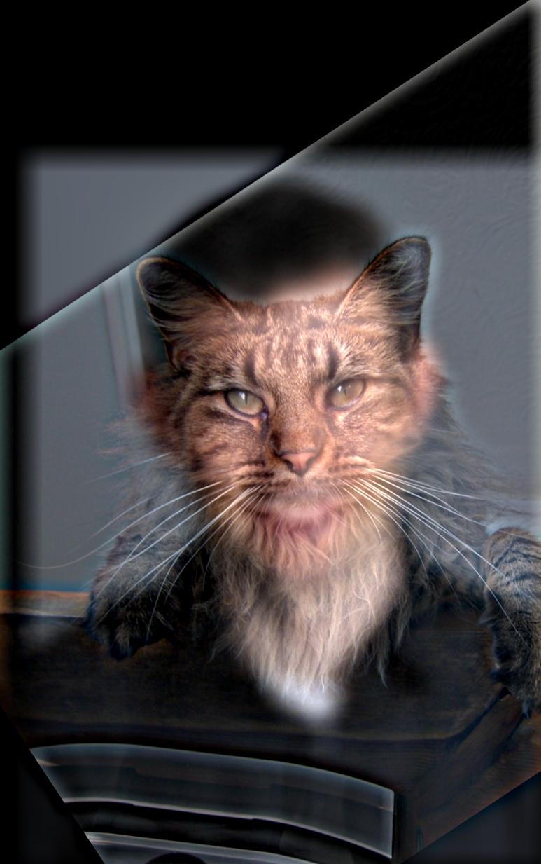
This part, I will go through the step to create hybrid image using following two image professor Derek and cat nutmeg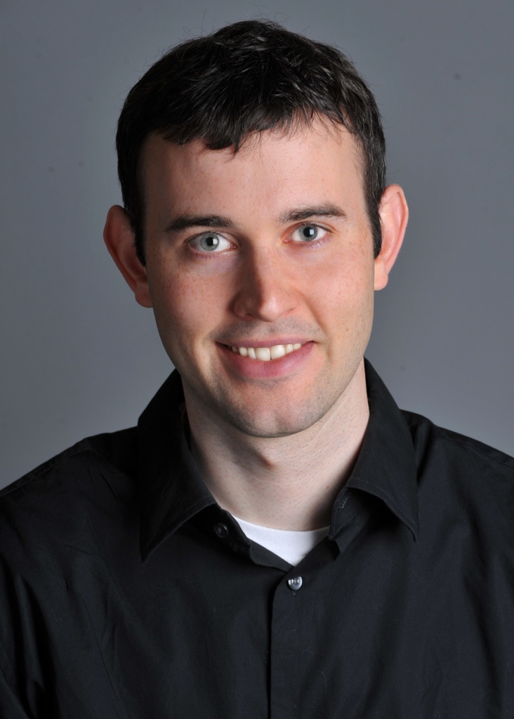
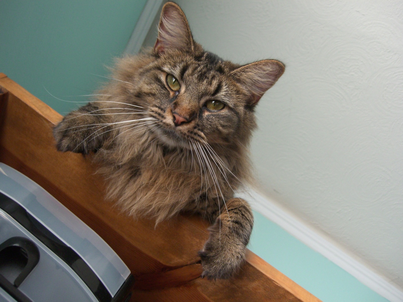
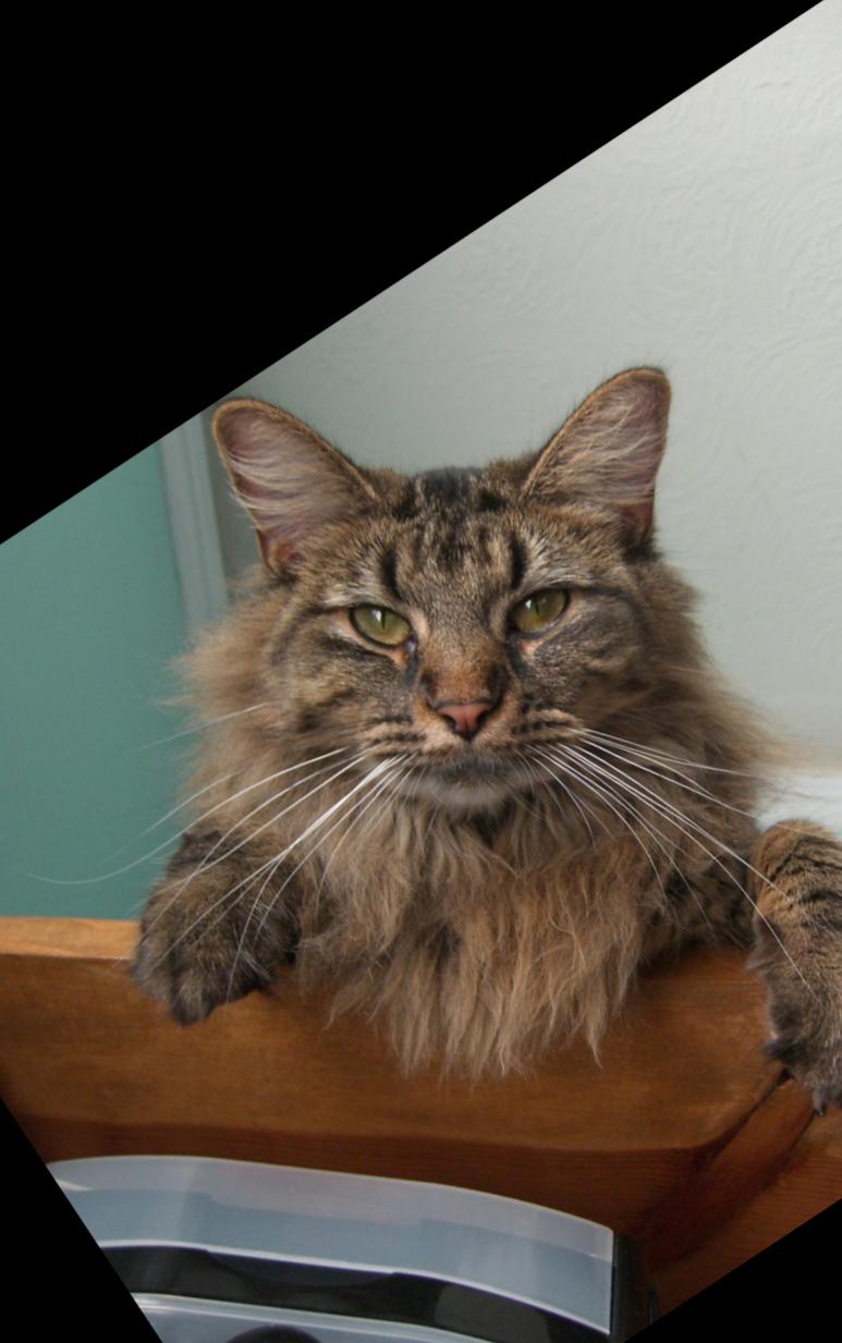
Step 1: aligned the image
We will first need to align the image so two image can overlap well in hybrid image Here we will rotate nutmeg.jpg so the cat face and professor's face can align. I also adjust the sizes of two images.
Step 2: Filter Image
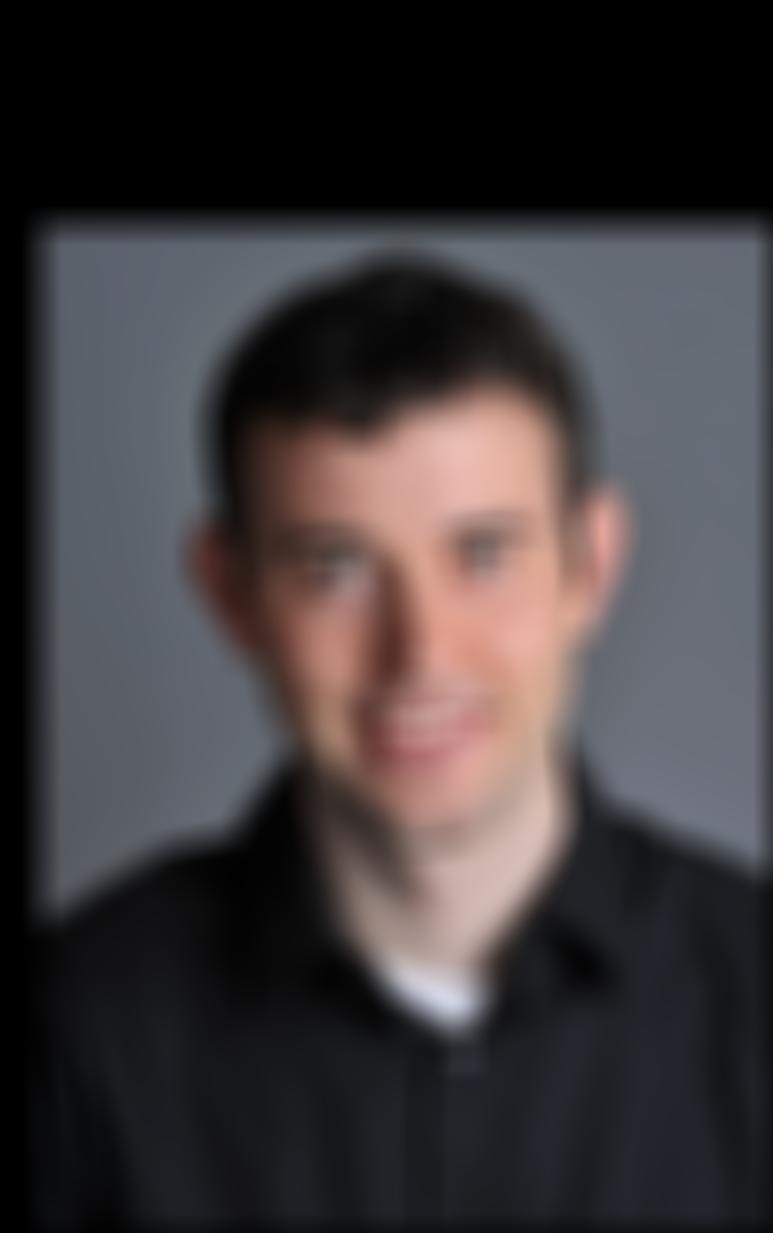
For image we want to see in close up, we will need to extract the high frequency of that image. To do that, we apply high-pass filter on one image. Here we will apply high-pass filter on the nutmeg.jpg. Then we apply low-pass filter on the other image.
low-pass filter can use gaussian filter
high-pass filter computed by subtracting the Gaussian-filtered image from the original.
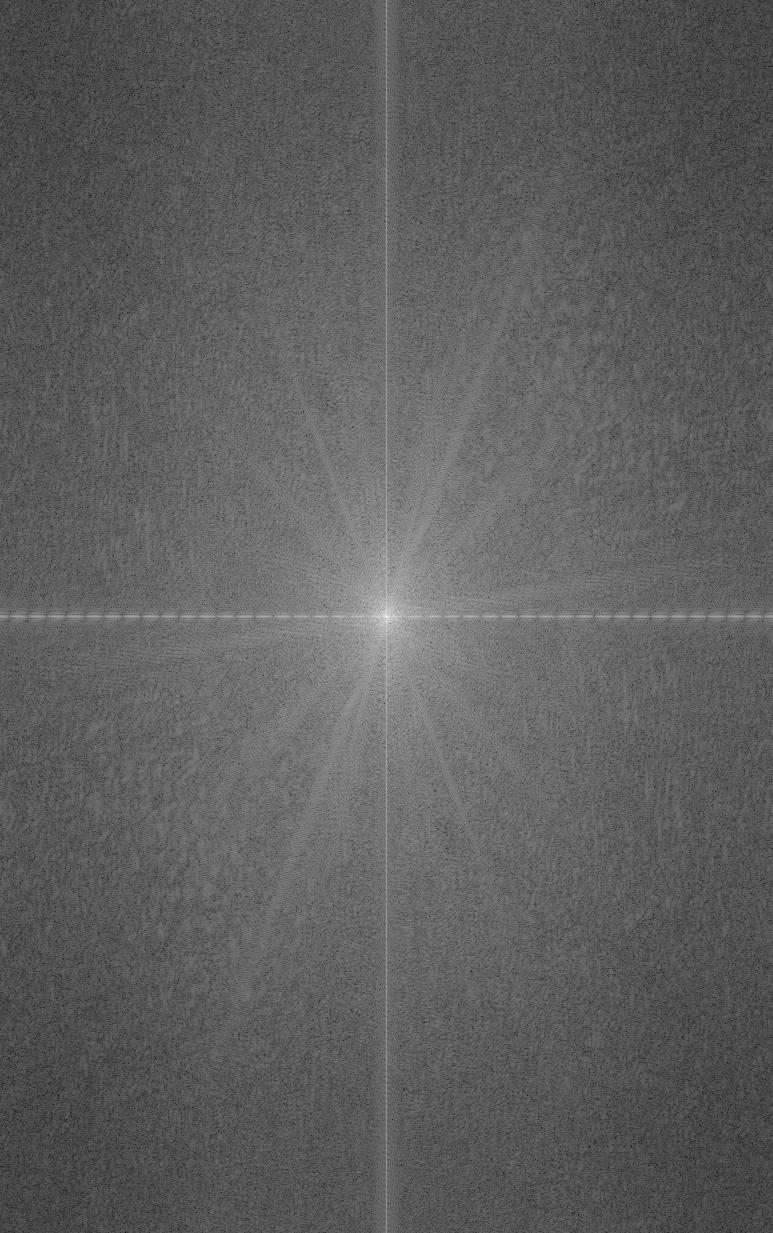
Step 3: Merge two image
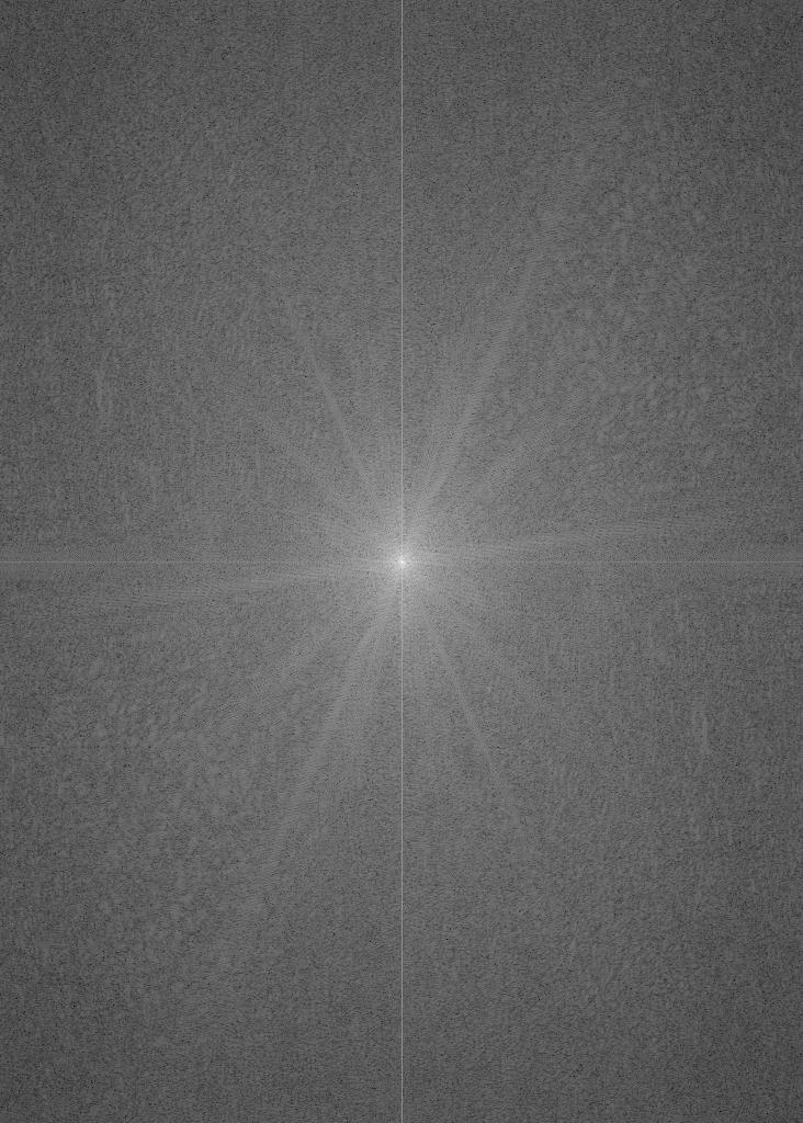
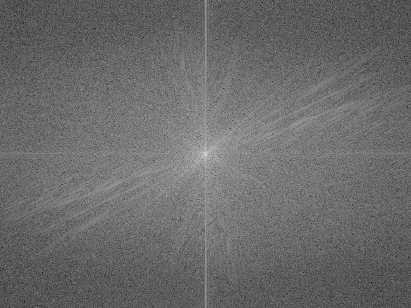
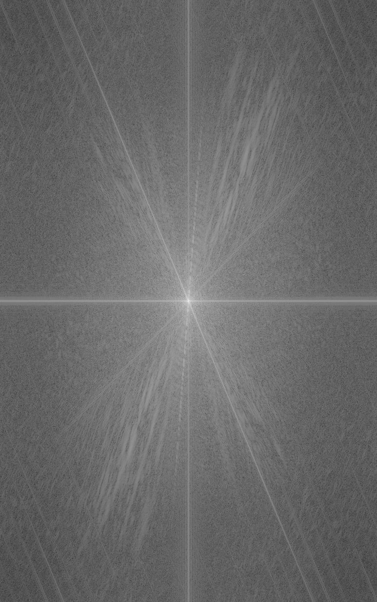
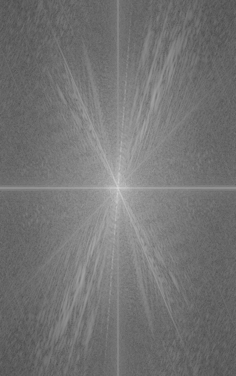
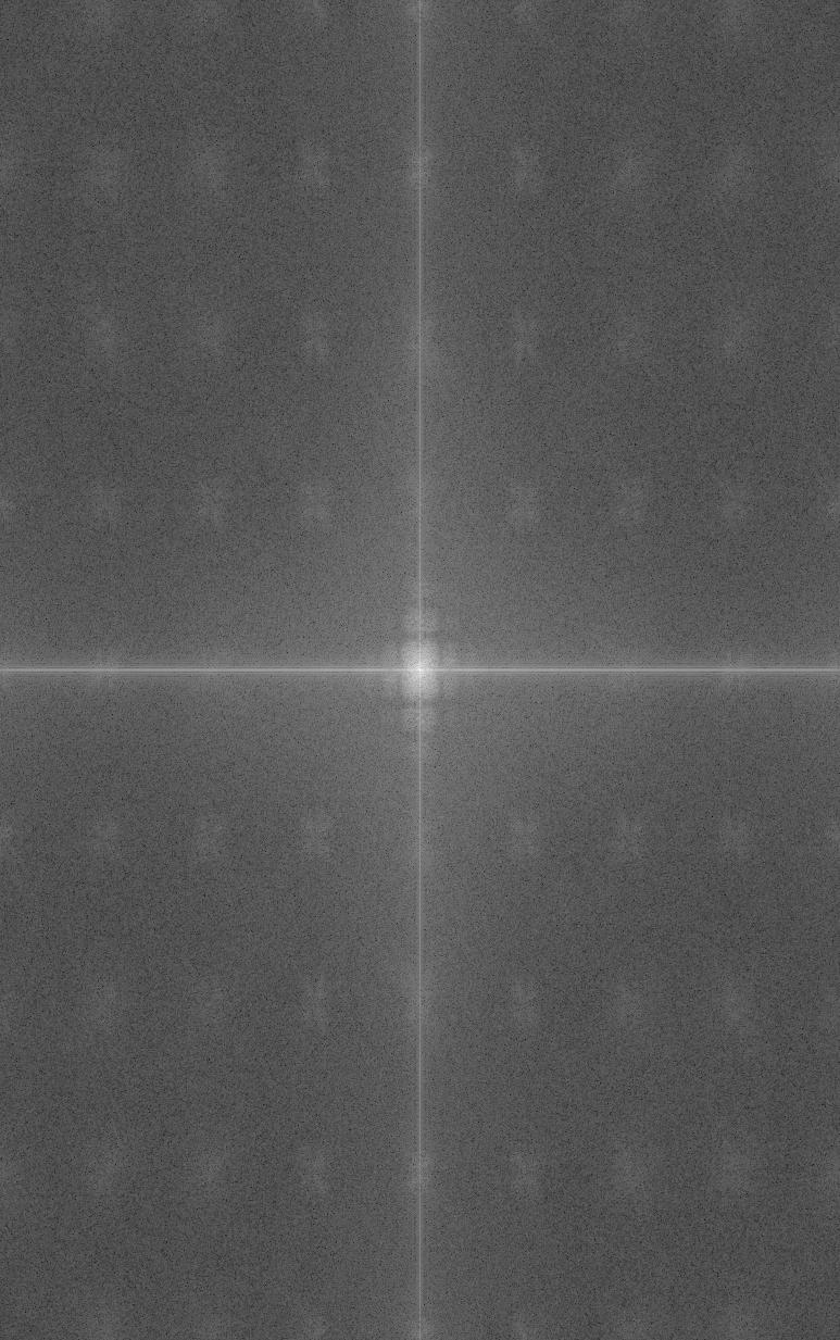
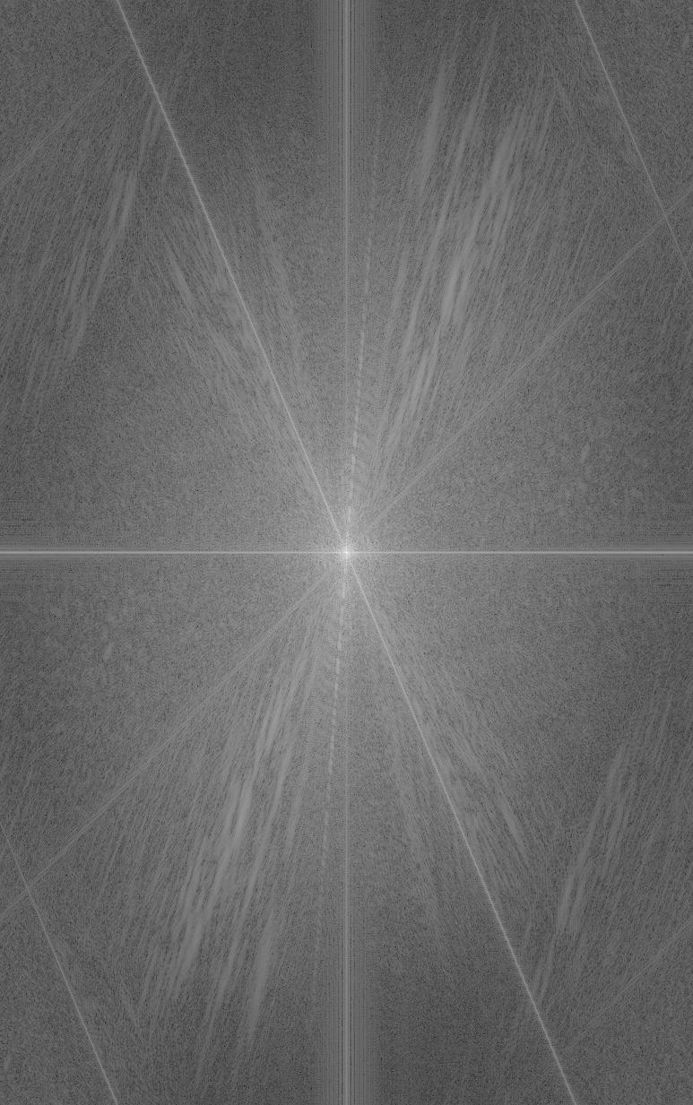
Finally we will add low-pass filtered image to high-pass filtered image to create hybrid image. Here I use sigma1 = 80, sigma2 = 30 for image 1 and image 2 respectively. From the fourier frequency image, we can see we merge the high-low freuqency from two images.
Other hybrid image examples

2.3: Gaussian and Laplacian Stacks
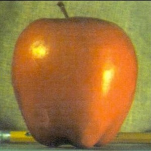
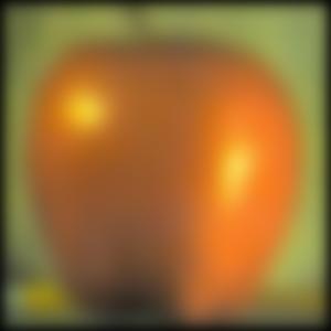
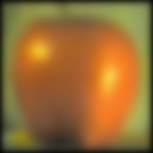
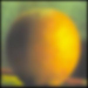
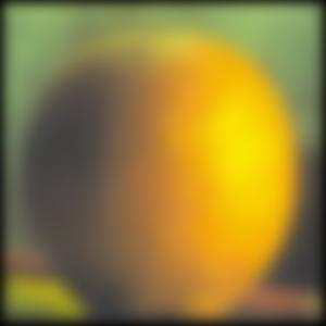
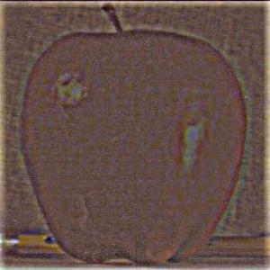
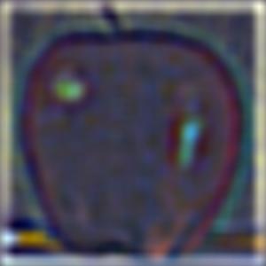
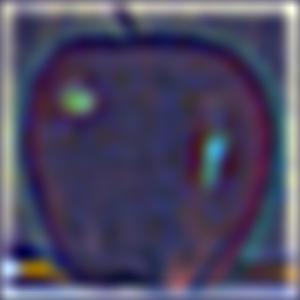
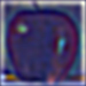
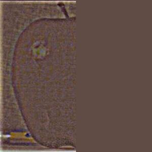
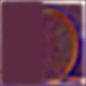
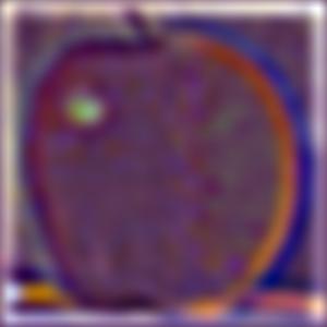
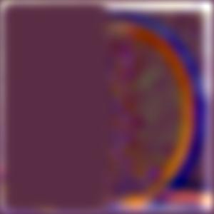
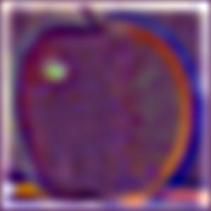
Gaussian Stack for apple (sigma=100, ksize=15)

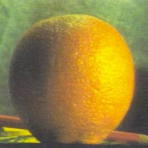
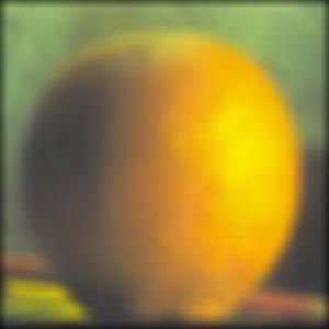
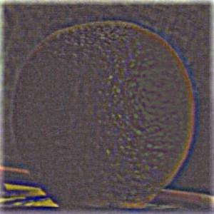
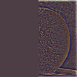
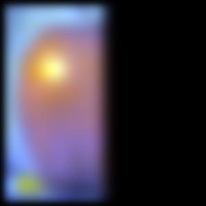
Gaussian Stack for orange (sigma=100, ksize=15)


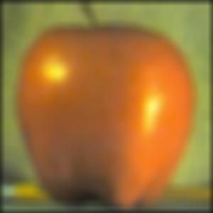
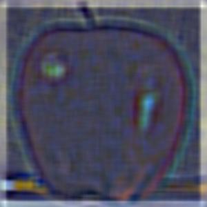
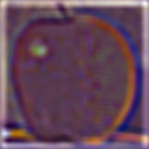
Laplacian Stack for apple
Note: Laplacian Stack share same lowest level image as Gaussian Stack
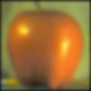
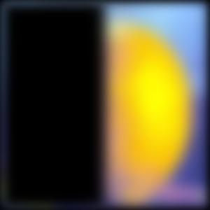
Laplacian Stack for orange
Gaussian Stack for the mask
Now we can apply build gaussian stack for the mask. Then we apply each level's blurred mask to corresponding level of Laplacian stack of apple and orange.
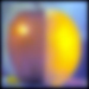
Finally, we collpase the combined stack to create the final blending image.
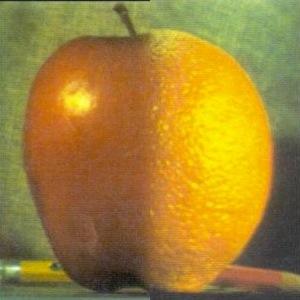
Part 2.4: Multiresolution Blending