Part A
Part 0: Setup
All the embeddings I generated: ['a high quality picture', 'an oil painting of a snowy mountain village', 'a photo of the amalfi coast', 'a photo of a man', 'a photo of a hipster barista', 'a photo of a puppy', 'a photo of a cat', 'a photo of dog fighting a cat', 'an oil painting of people around a campfire', 'an oil painting of an old man', 'a lithograph of waterfalls', 'a lithograph of a skull', 'a lithograph of book', 'a lithograph of a mountain', 'a lithograph of cat', 'a lithograph of a river', 'a man wearing a hat', 'a high quality photo', 'a rocket ship', 'a pencil', 'a photo of New York', 'a photo of mountains', 'a painting of sunflowers', 'a painting of village', '']
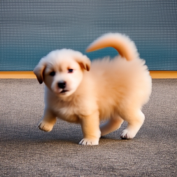
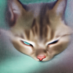
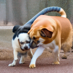
Here is the prompt I used for part 0, prompts = ['a photo of a puppy', 'a photo of a cat', 'a photo of dog fighting a cat']
seed = 100
num_inference_steps = 6
num_inference_steps = 20
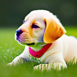
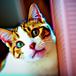
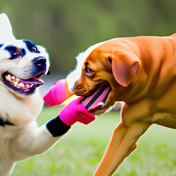
By comparing two inference steps: we can see longer inference step can produc image with more colors and details, we can see that by comparing the two cat image, num_inference_steps=6 produces really blur cat image while num_inference_steps=20 produce fine-detailed cat It takes longer to generate correct picture for complicated prompts like a photo of dog fighting a cat. With num_inference_steps=6, there is almost no signs of fighting and with num_inference_steps=20, we can the see the fighting but it is not a dog and a cat fighting.
Part 1: Sampling Loops
1.1 Implementing the Forward Process
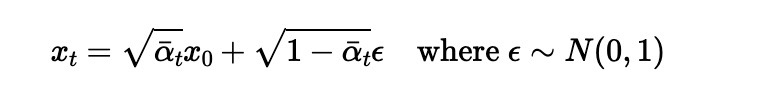
Using above formula, I implemented noisy_im = forward(im, t) function

.png)


1.2 Classical Denoising


1.3 One-Step Denoising


1.4 Iterative Denoising
On the ith denoising step we are at t = strided_timesteps[i], and want to get to t = strided_timesteps[i+1] (from more noisy to less noisy).
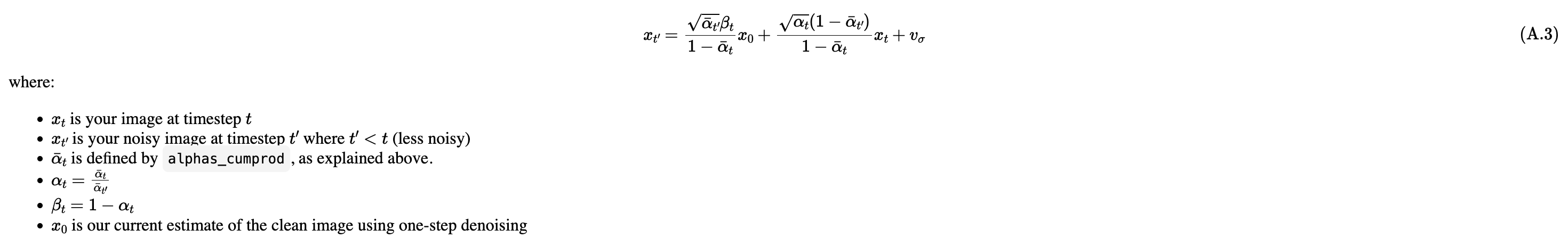
Using above formula we can create function
def iterative_denoise(im_noisy, i_start, prompt_embeds, timesteps, display=True):


1.5 Diffusion Model Sampling
In iterative_denoise function, we set i_start = 0 and passing im_noisy as random noise.


1.6 Classifier-Free Guidance (CFG)

Use above formula combine with iterative_denoise function from Q4, we can create function
def iterative_denoise_cfg


1.7 Image-to-image Translation
run the forward process to get a noisy image, and then run the iterative_denoise_cfg function using a starting index of [1, 3, 5, 7, 10, 20] steps. with the conditional text prompt "a high quality photo".


1.7.1 Editing Hand-Drawn and Web Images
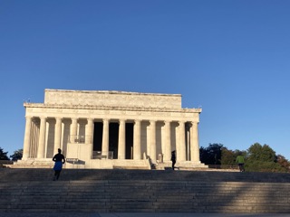
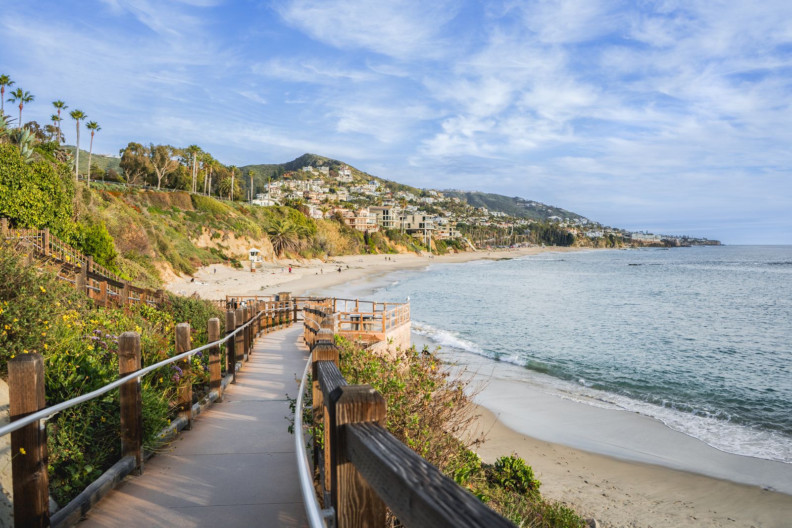
Web Image


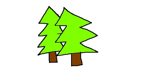
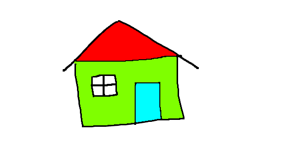
Hand-Drawn


1.7.2 Inpainting

Use above formula combine with def iterative_denoise_cfg to create inpaint function


1.7.3 Text-Conditional Image-to-image Translation
Prompt = a rocket ship


Prompt = a photo of mountains


Prompt = a photo of New York


1.8 Visual Anagrams

above algorithm plus iterative_denoise_cfg create visual_anagrams function


1.9 Hybrid Images
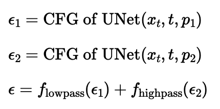
above algorithm plus iterative_denoise_cfg create make_hybrids function
Used Gaussian Blur to create lowpass, and subtract from lowpass to create high pass


Part B
Part 1: Training a Single-Step Denoising UNet
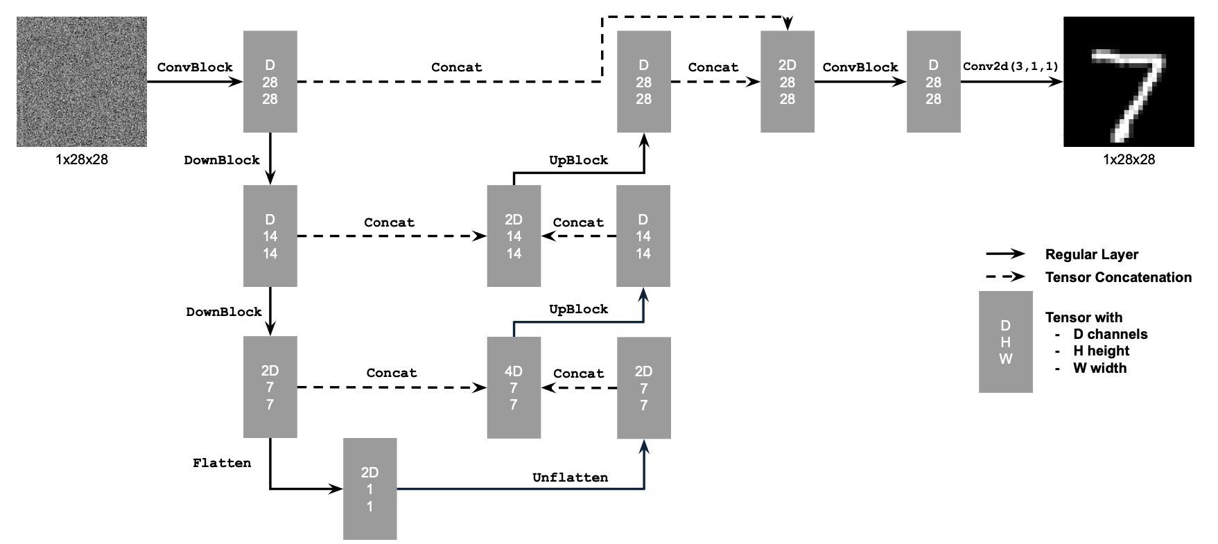
1.1 Implementing the UNet
Here is the structure of simple Unet
1.2 Using the UNet to Train a Denoiser

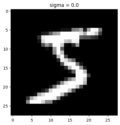
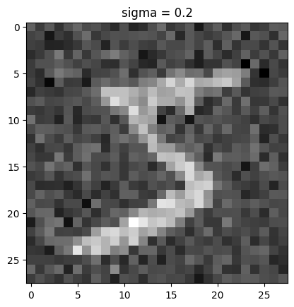
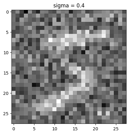
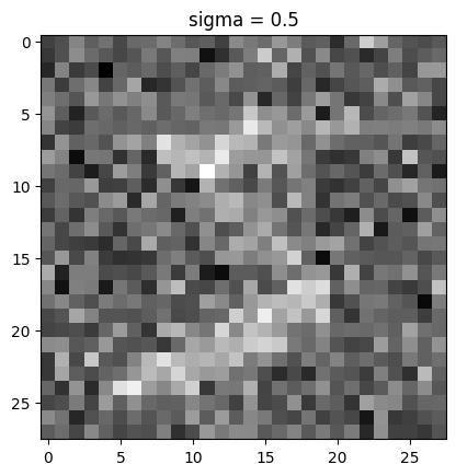
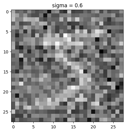
Using above formula, we can create different noise level for each image
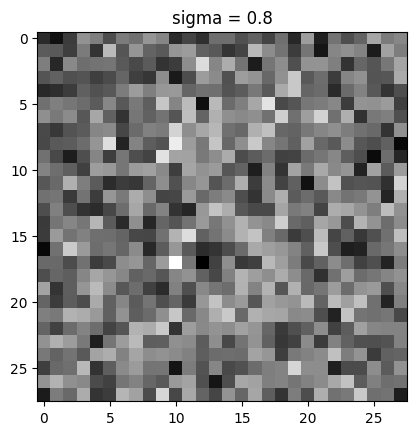
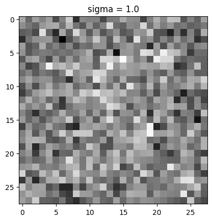
visualization of the noising process using sigma = [0.0, 0.2, 0.4, 0.5, 0.6, 0.8, 1.0]
1.2.1 Training
epoch 1


epoch 5


1.2.2 Out-of-Distribution Testing


Denoiser performs relatively well when noise level less or close to 0.5. It's started to struggle to denoise the image when noise level become 0.8 or 1.0
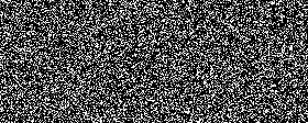
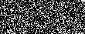
1.2.3 Denoising Pure Noise
epoch 1


epoch 5


The general pattern of Denoising Pure Noise model is that it always produe a general shape that could possibly be any number. A blob of cloud in the middle
Q: What relationship, if any, do these outputs have with the training images (e.g., digits 0–9)? A: these outputs (a cloud of pixels) seems encampass all posible training images
Q: Why might this be happening? A: I think one reason might be it was trained with all 10 digits and it can't observe any strong direction to one digit during training since the input is pure noise, it decided to produce the output that can potentially match all 10 digits in some way so a cloud of pixels is always predicted. No time conditioned or class conditioned, the model tried to find "average point" for all possible output.
Part 2: Training a Flow Matching Model
2.1 Adding Time Conditioning to UNet
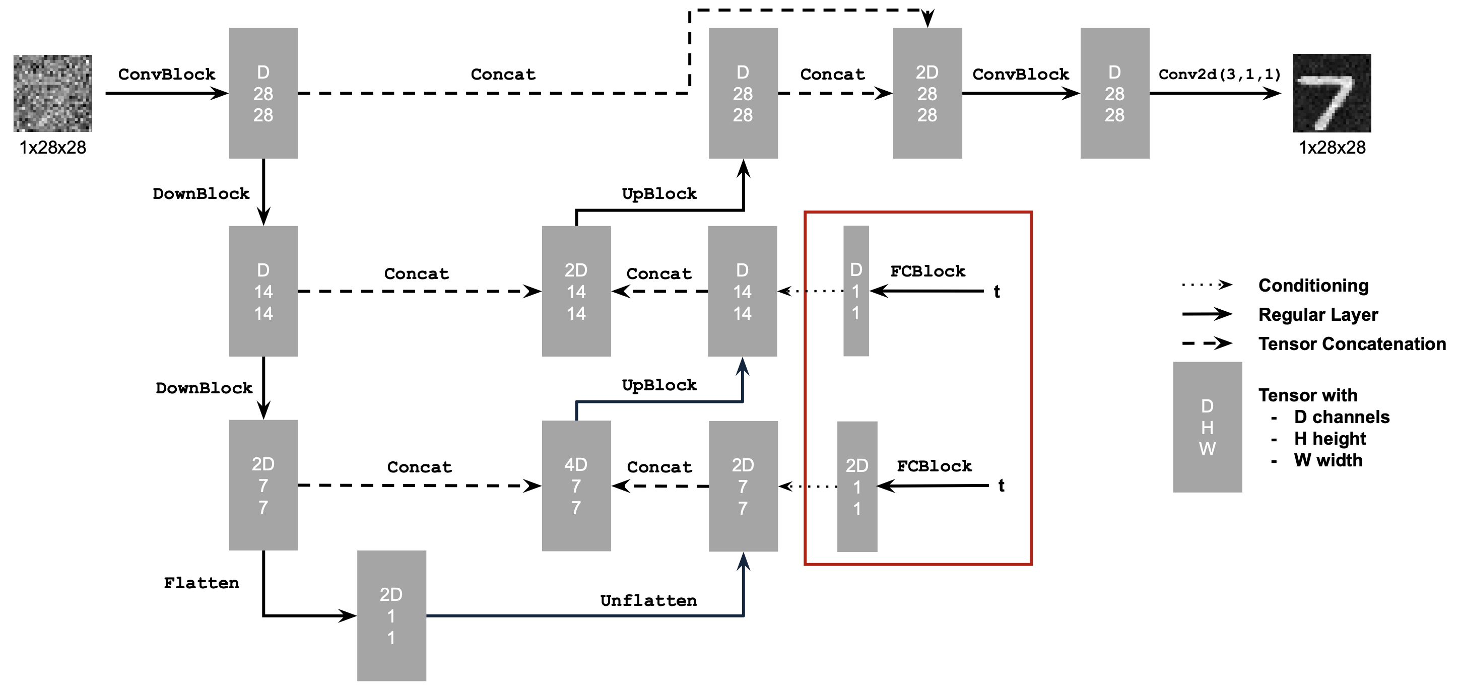
Use above structure to build time-conditioned Unet
2.2 Training the UNet
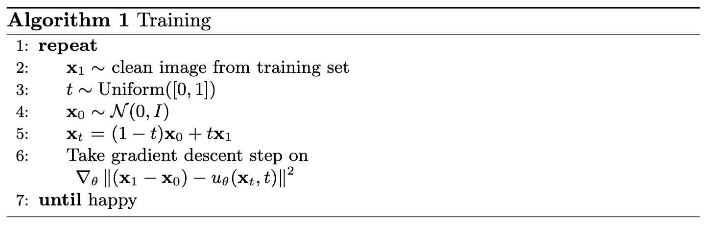
We will train time-conditioned model with following algorithm
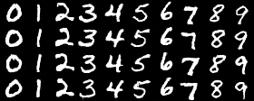
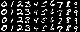
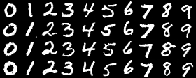
2.3 Sampling from the UNet
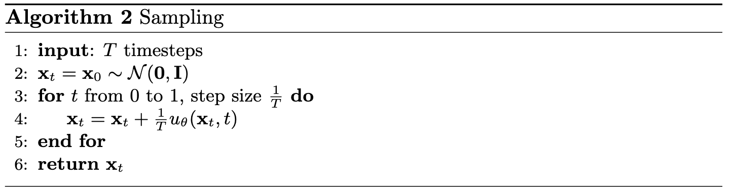
We will generate time-conditioned model output with following algorithm


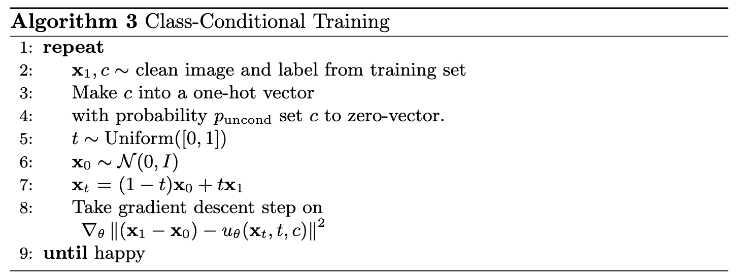
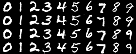
2.4 Adding Class-Conditioning to UNet
Adding classes during training by adding two more FCBlock with input class-conditioning vector, you make it a one-hot vector instead of a single scalar.
Because we still want our UNet to work without it being conditioned on the class (recall the classifer-free guidance you implemented in part a), we implement dropout where 10% of the time we drop the class conditioning vector c setting it to 0.
2.5 Training the UNet
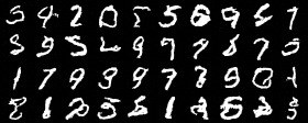
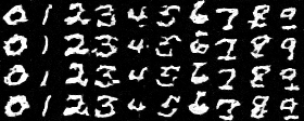
2.6 Sampling from the UNet
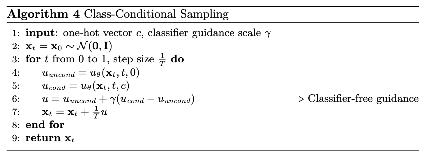
Now we will sample with class-conditioning and will use classifier-free guidance with guidance_scale = 5
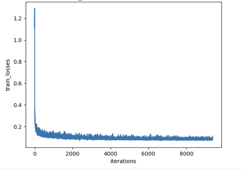
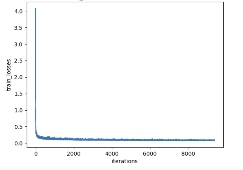
training visualization with scheduler

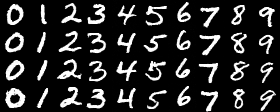
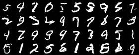
training visualization without scheduler

To compensate the loss of learning rate scheduler, I did the following
I added gradient clipping to prevent gradient explosion
torch.nn.utils.clip_grad_norm_(unet.parameters(), max_norm=1.0)
I also reduce learning rate to 5e-3 to avoid overshoot
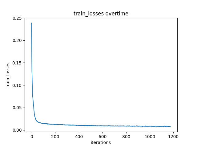
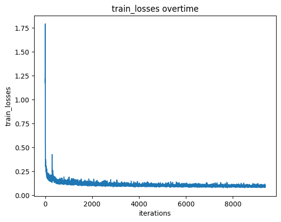
There is no big difference in training losses
By comparing the visualizations, we can see there is no significant difference between using scheduelr and not using scheduelr